PiBrush — Painting with the Pi and XLoBorg
Turning an accelerometer into a paint brush with Raspberry Pi
Fred Sonnenwald, September 2013
[Featured in The MagPi, December 2013]
Contents
1. Introduction
Two weeks ago we participated in the Ideas Bazaar promoting Open Culture Tech, which I've translated to myself as a promoting how we can take finer control of technology for ourselves using low-cost and open technologies. "The proof is in the pudding" though, and actually demonstrating the point is a much more powerful argument. To this end we prepared our exhibit to show off various gizmos and widgets, including those based around Raspberry Pis. My contribution has been the PiBrush.
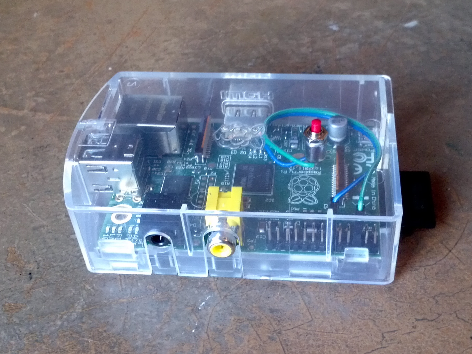
The PiBrush is an interactive art and technology exhibit (a very grand name for something so small) that simulates flicking paint off the end of a paintbrush onto canvas — as Jackson Pollock famously did in the 1940s and 50s. It utilizes two Raspberry Pis (one Model B and one Model A), a PiBorg XLoBorg accelerometer, a battery pack, a display, and two Wi-Fi dongles. The Model A is held by the user and waved around. It collects acceleration data with the XLoBorg, which it then transmits via Wi-Fi to the Model B, which processes the data collected into paint droplets and displays them on the screen, connected via HDMI.

|
|
|

Since the Bazaar, we've also added a physical reset button to save the current canvas and reset it to blank.
2. Programming
The hardware for this project is fairly straight forward. The XLoBorg plugs directly into the GPIO pins as a block, and a GPIO button is just a button connected between the ground and a GPIO pin — we've used BCM pin 17 or board pin 11. The software is where the challenge lies.
I developed the code from scratch, and doing so required a variety of knowledge. While I'd rate it as intermediate to advanced code to write, I'm hoping to shed enough light on it here that it is only beginner to intermediate to understand. The only real requirements are some basic familiarity with the Python programming language, networking (IP addresses), and basic Physics.
First, what code. The code is available on GitHub. This will always be the latest version. There's the python file accel_client.py which runs on the Model A and there's accel_server.py which runs on the Model B. The former reads in off the sensor and sends it across the network, the latter recieves the data, does processing, and displays the output on the screen.
2.1. accel_client.py
The client script is fairly straight forward. There are two unique points to consider though. Reading in the accelerometer data and the networking code. First though, we import the necessary libraries.
import socket
import XLoBorg
import time
import os
socket is for networking and XLoBorg, the accelerometer. time is used to for its sleep function and os to read in the server's IP address. So let us first setup for the networking.
# network stufff
server = os.getenv('SERVER', 'modelb')
port = 5005
Lines 7 and 8 define the IP address (or hostname) and destination port of the
server. You'll notice os.getenv is used. This checks for what are called
environment
variables. They're set before the program is run. If there's nothing found
it defaults back to 'modelb' in this case though. I've arbitrarily picked out
the port number. Generally any number over 1024 is fine though.
The XLoBorg has its own specific initialization function to be run at the start of a program using it. This uses the library to start communicating with the accelerometer over the I2C bus.
# setup for the accelerometer
XLoBorg.printFunction = XLoBorg.NoPrint
XLoBorg.Init()
Next, the outgoing socket is created. Sockets are the mystical term used to describe the connector that programs use for talking to each other over the internet. They come in different forms, we're using a UDP socket, also known as a Datagram socket. The special ability of these that we're taking advantage of here is that UDP is simple and stateless. It's easy to setup and the Model A can continually send and it doesn't matter what the Model B does. That makes for conveniently robust communication in this scenario.
# make the socket connection
sock = socket.socket(socket.AF_INET, socket.SOCK_DGRAM)
Afterwards, the main program begins as we enter an infinite loop — we want to continually read the accelerometer and send that information off. Line 17/18 are used to construct the outgoing message. It conists of three comma seperated, signed, floating point values which are fed from the special XLoBorg ReadAccelerometer function. (See String Formatting Operations for details on this.) sock.sendto then sends the message and then time.sleep causing Python to wait for a small interval. Then it all starts again — about 200 times a second.
while True:
    message = '%+01.4f,%+01.4f,%+01.4f' \
            % XLoBorg.ReadAccelerometer()
    sock.sendto(message, (server, port))
    time.sleep(0.005)
That's it. Not so bad. A nice warm up...
2.2. accel_server.py
The server script is where the real meat of the programming is as it handles the simulation and display. Similar to accel_client.py, necessary libraries are first imported.
import socket
import select
import pygame
import time
import numpy
import math
import datetime
import random
import os
import RPi.GPIO as GPIO
socket we've already met, but select is new, and related. It's used to avoid what's called blocking, which is when the program is forced to wait for new data. Using select, the network code becomes non-blocking, which allows the program to function even if the client isn't transmitting any data. Pygame is a the library used for drawing on the screen. numpy is used for fast array operations to help speed up program execution — the RaspberryPi isn't the world's fastest computer and every little helps.
math contains the functions like sin and cos which we use to handle some of the translation from where the accelerometer is to where the paint is on the screen. datetime is a bit of code that got accidentally left in from an old version — oops! (It was used to print the current date on the screen during debugging to tell if the program was frozen or not.) random is used to generate, as it sounds, random numbers. Finally RPi.GPIO is used to talk with the GPIO pins.
2.2.1. Initialization
# ==============
# initialization
# ==============
Next comes a lot of boring and tedious bits of code which I've classed under initialization. These are various pieces of code that need to be run just once to get things started.
# port to listen on
port = 5005

# setup networking
sock = socket.socket(socket.AF_INET,
        socket.SOCK_DGRAM) # UDP
sock.bind(("0.0.0.0", port))
sock.setblocking(0)
First there's the network code. This will look familiar. It's the flip side of
what was done on the client. We define the network port to listen on and then
create a socket. Then we tell the socket to listen using the .bind()
function. 0.0.0.0 in this case tells it to listen on all network interfaces
(so you could use Ethernet or Wi-Fi). Then .setblocking() is needed for that
non-blocking thing I mentioned before.
# directory for saves
SAVEDIR = os.getenv('SAVEDIR', '.')
os.getenv is used again, the first of several times. This time it's used to
set a directory to store save files in, and otherwise defaults to '.', which is
the current working directory (the folder you were in when you started the
program).
# setup GPIO input for reset
GPIO.setmode(GPIO.BCM)
GPIO.setup(17, GPIO.IN, pull_up_down=GPIO.PUD_UP)

# variable to store button state
button = 0
The above code initializes the GPIO for input. .setmode() says we'll be using the Broadcom pin names. .setup then says we're looking for input on pin 17. It also specifically tells the chip to use the internal resistor on the pin so that there's no floating. (Here is a pretty good article to which explains floating, some interesting extra reading.) The last thing is the button variable which is used to indicate whether or not the button hooked up to the GPIO has been pushed or not. By default it's not been so it starts at 0.
# screen solution
XRES = int(os.getenv('XRES', 1920))
YRES = int(os.getenv('YRES', 1080))

# setup display
pygame.init()
screen = pygame.display.set_mode((XRES, YRES))
# reset to white
screen.fill((255, 255, 255))
# push white
pygame.display.flip()
Then comes screen initialization. First we read in the X resolution (XRES)
and Y resolution. (YRES).
int() is used to
convert the string that getenv returns into a number we can do calculations
with later. After getting the resolution, we initialize pygame and set the
display mode with it. By default the screen is black, but I think a nice
white canvas is preferable so we .fill() the screen with white. (255, 255,
255) is 0-255 (red, green, blue). All colors combined = white (think prisms).
By default pygame writes to a buffer section of memory, so .flip() is
required to tell it to display the current buffer. (A second buffer is then
availble to draw on until the next flip — this is called double buffering.)
# length of moving average array
AL = 20

# accelerometer storage for moving average
AXa = numpy.zeros((AL, 1))
AYa = numpy.zeros((AL, 1))
AZa = numpy.ones((AL, 1))

# array index for accelerometer data
Ai = 0
Next we create the variables used for storing the raw accelerometer data — that's the AXa, AYa, and AZa variables. There's a numpy array for each direction, X, Y, and Z. X is into the screen, Z down it and Y across. But why arrays? Surely a single reading should be in a single variable? Normally that would be the case, but we're going to use something called a moving average (MA) to filter the input data.
An MA is the average of, in this case, the last 20 readings. Some sort of filtering is almost always necessary when dealing with the sort of analog input data that comes from an acceleromter to prevent sudden jumps in the readings (e.g. you knocked it) from having an undue impact on the processing. An MA is a convenient and easy way to do it. We simply input The current reading at index Ai and then increment Ai until it exceeds AL, then wrap it back around. You'll see this in the code later. I use numpy here because they execute very quickly (read: effeciently) and there are handy functions to make things simpler. Like .ones() to initialze all of AZa to a value of one — there's always by default 1G of gravity downwards.
After dealing with the accelerometer directly are declarations for those variables dealing with gravity. GX, etc., store the best (most recent) guess of what direction gravity is in, as once we start moving we have a combined acceleration of gravity plus the user's movement. We need this to subtract gravity back out so we know how the user is moving. Ideally this would be done with a gyroscope, but we don't have one of those so we make do.
# store gravity when fast is detected.. GX = 0 GY = 0 GZ = 1 # polar gravity PGR = 0 PGA = -math.pi/2 PGB = 0 # screen gravity PSGR = 1 PSGA = -math.pi/2 PSGB = 0 # accelerometer values AX = 0 AY = 0 AZ = 0 # rotated for screen accelerometer values GAX = 0 GAY = 0 GAZ = 0PGR, etc., store the equivalent polar coordinates of the gravity estimate, where R is the radius to the point from the origin, and A and B are the angular rotation about the Z and Y axis. The polar coordinates are used for the actual subtraction as subtracting the gravity vector from the current acceleration vector is very easy like this — it's an extension of the regular subtraction of vectors.
PSGR are the polar coordinates of gravity in the screen, which is an accleration field that's always downwards. If you consider that the Model A might not be parallel to the screen while being waved about (e.g. it's held rotated) then we need to rotate the acceleration field it experiences back to screen normal. I'm actually not entirely sure about this — this was all new to me when I was writing it, so this is just a guess really. It seems to work though so I've left it in. In my experience most projects like this have fiddly bits like this.
AX etc. store the result of the moving average of the acceleromter data. GAX etc. store the current acceleration as from AX but rotated correctly for the screen.
last_G = 0 # timing information last_time = time.time();last_G stores the time at which the last estimate of the direction of gravity was taken. last_time stores the time at which the last loop was executed. This is used for estimating distance the brush has travelled as part of a process called twice integration. You think someone would have written up a nice simple explanation of this, but nothing turns up after a quick Google. This is a somewhat high level explanation of what's going on, and this is a bit simpler, but I'm not terribly happy with either explanation. I'll try and simplify it a bit, or at least put it a bit more concisely.
Imagine you're in a car traveling down the motorway at 100 kph. In one hour you will have travelled 100 km. Easy? That's simple integration, going from velocity to displacement. Acceleration though, is the rate of change in velocity, e.g. the speed at which the needle of the speedometer in the car climbs. So now imagine accelerating at 1 kph per second, after 10 seconds you'll be going 10 kph faster, so instead of 100 kph you're now going 110 kph. Apply that to the distance you've travelled and you have twice integration. (Fun fact: if you kept up that acceleration, after an hour you'd be going 3,700 kph and would have traveled 36,370 km. Or almost around the Earth.)
# brush info
BX = 0 # position
BY = 0
VX = 0 # velocity
VY = 0
P = 0 # amount of paint on brush
S = 0 # distance brush has traveled
last_stroke = 0
This next bit of code initializes the variables regarding our virtual paintbrush. BX and BY for the position on the screen — no Z because it's only going up and down. VX etc. for it's velocity, or speed. P to keep track of how much virtual paint is left on the brush, and S to keep track of how far the brush has travelled - this is used in determining how far apart the paint splatters ought to be. last_stroke is the time at which we last painted.
# seed random number generator
random.seed(time.time())
This last bit of code initializes the random number generator with the current time. Without this, it would be possible to get the same random numbers over and over each time the program was run. We use the random numbers for picking out the paint color each stroke.
2.2.2. Functions
# =========
# functions
# =========
If you don't know, a function is a bit of code written in such a way that it can be executed from different places in the main program. Each call you can pass different arguments (input parameters) that will be operated on and a new result returned. If you already know this that's handy. There are three functions which I've written for use in accel_server.py.
def polar(X, Y, Z):
    x = numpy.linalg.norm([X, Y, Z])
    if (x > 0):
        y = -math.atan2(Z, X)
        z = math.asin(Y / x)
    else:
        y = 0
        z = 0
    return (x, y, z)
polar takes a Cartesian X, Y, and Z coordinate and returns the equivalent
polar coordinates. It's used several times later to make the conversion, as
previously mentioned, as part of rotating gravity. I've based it off the code
in this forum
thread.
def cartesian(X, A, B):
    x = 0 # don't bother - isn't used
    y = X * math.sin(B) * math.sin(A)
    z = X * math.cos(B)
    return (x, y, z)
cartesian as you might suspect does the opposite of polar, taking the
distance X and rotations A and B and turns them back into Cartesian
coordinates. As this code is only used as part of getting coordinates ready for
the screen, x, as the coordinate into the screen, is permanently set to 0. This
is an optimization to help the code run better on the Pi. The code here is
based on this
explanation of Cartesian and polar coordinates.
def savereset():
    filename = SAVEDIR + os.sep + ("%i.png" % time.time())
    pygame.image.save(screen, filename)
    screen.fill((255, 255, 255))
The last function, saverest is called when either the 'R' key is pressed on
the keyboard or the GPIO button is pressed. It (you may notice a pattern in the
function names) saves the screen and then resets it back to white. filename
is created as the previously defined SAVEDIR plus os.sep which is a fixed
variable as the file system serpator - '/' under Linux. ('\' under Windows.)
After the save path comes the actual file name, which we want to be unique so
that we don't overwrite an old file. We also don't want to have to stop for
user input in case there's no keyboard.
In this scenario I've found a Unix timestamp to be the easiest way of doing this. It's simply the number of seconds since Jan. 1, 1970, but it's always going up and unless someone invents time travel won't repeat. You may have realized though that as the Pi doesn't have a real time clock, it may indeed count the same time over and over. A weakness that will have to be accepted. Besides, what are the odds someone would reset the screen at exactly the same number of seconds since the Pi was turned on twice? (A proper way to fix this though would be to check for an existing file first.)
2.2.3. Main program
# ============
# main program
# ============
That's the functions over, now onto the main program! Interesting things start to happen. Almost. 3 more variable declarations that in this funny spot first though. They ended up here though because they specifically have to do with code loops.
fast = 0
notfast = 0
running = 1
while running:
fast is used to indicate whether or not the Model A is currently being waved around and is trigged when acceleration starts. It's the start of a brush stroke. notfast is an indicator of the opposite, the amount of time Model A has not been accelerating. This isn't a binary true or false situation as you might suspect as there's a quick point in time when there's no acceleration. This time is the difference between lifting up on the gas pedal in the car and pressing brake pedal to slow down. Paint droplets shouldn't stop being deposited on the screen between the end of starting to wave and the beginning of stopping to wave the Model A as that's unrealistic.
running is what it sounds like and is used to keep the program continually looping in a while loop. When we want to quit we set running to 0, the loop finishes and then the program exits.
The main program loop consists of three phases. Phase 1 consists of basic tasks that need to be done over and over. Phase 2 consists of reading the accelerometer data and pre-processing it. Phase 3 consists of manipulating the paintbrush and canvas.
2.2.3.1. Phase 1
    # move time forward
    dt = time.time() - last_time
    last_time = time.time()
The first thing to be done each loop is to move time forwards. Ideally
execution time for each loop is identical and dt (change in time) is the
same. However, something may interrupt, cause a bit of lag, or some if
statement may be skipped either increasing or decreasing execution time of the
loop. For something that moves on the screen this is bad, so by knowing how
long it's been since the last update we can know how far to move things, i.e.,
distance = velocity * time.
    # no changes made to the screen so far
    draw = 0
draw is a marker to tell us whether or not to .flip() the screen later. If we
don't need to, we won't. This saves some CPU time, and is one of the reasons
dt is important.
The next two bits of code deal with input. The first is keyboard input handled though PyGame. The second is GPIO input from the push button we installed, which we handle manually.
    # check for keyboard input
    event = pygame.event.poll()
    if event.type == pygame.QUIT:
        running = 0
    elif event.type == pygame.KEYDOWN:
        if event.key == pygame.K_q:
            running = 0
        elif event.key == pygame.K_r:
            savereset()
            draw = 1
.poll() performs an instantaneous check of the keyboard (and for example
joystick if we had one of those) and stores it in event. event then
contains all the information about what was found in the poll. First is what
type of event is happening? There's a special pygame.QUIT type, which is
triggered a number of different ways, clicking the X button in a window, by
the kill command, etc. It checks all of those so that we can quit nicely. In
general though we don't expect this to happen.
pygame.KEYDOWN is a regular keypress. Once we know it's a keypress, we can check which key has been pressed. If it's the Q key we indicate we want to quit but setting running to 0. If it's the R key we save the screen, reset it, and then set draw to 1 so that we know to .flip() later.
    # check for GPIO input, but because it's a
    # pull down (goes from 1 to 0 when pressed)
    # flip logic
    button_now = not(GPIO.input(17))
    if button_now == 1 and button == 0:
        # the button was pressed
        savereset()
        draw = 1
    button = button_now
The logic for the GPIO check is a bit more complex. Because the button
connects the pin and ground and the pin is in a pull up state, by default
.input() reads a 1. Which we would normally associate with it being pressed.
Therefore we use not() to flip a 1 to a 0 and a 0 to a 1. This way
button_now instead gives the sort of value we expect - 0 when not pressed
and 1 when pressed.
The other thing we have to consider is what happens when the button is pressed and held down. In this case we only want to trigger a save and reset once, not multiple times. That's why we check not only if the buttonnow is 1, but also that button is 0, i.e. in the previous loop it wasn't pressed. We then set button to buttonnow so that when we hit the next loop we know it was pressed and don't reset the screen.
2.2.3.2. Phase 2
    # ===================
    # networking & sensor
    # ===================

    result = select.select([sock], [], [], 0)
    if len(result[0]) > 0:
Now we check for sensor input over the network and pre-process it if there is.
This is the non-blocking magic I mentioned earlier. .select checks sock for
any new packets and puts them in result[0] (0 because you can select from
multiple sockets). When there's something the length of results[0] will be
non-zero and so we know to go to work. Doing it this way is potentially a
little buggy, but seems to be OK. It might be better replaced with a for loop.
        # read in data
        data = result[0][0].recvfrom(1024)
        a = data[0].split(",")
        AXa[Ai] = float(a[0])
        AYa[Ai] = float(a[1])
        AZa[Ai] = float(a[2])
        Ai = Ai + 1
        if Ai == AL:
            Ai = 0
data takes on the value of the first packet waiting. If you remember, it's a
comma seperated string with the X, Y, and Z values of acceleration from the
accelerometer on the Model A. We can use
.split() to
break it apart into an array of strings for each axis.
float() is used to
convert the string back into a floating point number (just like with int()
before), which we then store in the moving average array we initialized earlier
at index Ai. Then it's incremented and if it's at the array length AL we set it
back to 0. Remember that arrays start at index 0 so the last index is the is
the length minus one.
        # moving averages for acceleration
        AX = numpy.sum(AXa) / AL
        AY = numpy.sum(AYa) / AL
        AZ = numpy.sum(AZa) / AL

        # combined acceleration for
        # working out resting gravity
        A = math.fabs(numpy.linalg.norm([AX,
                AY, AZ]) - 1)
.sum() does what it says on the tin and returns the sum of all the values in
an array (it adds them all up). To do an average is the sum divided by the
number of elements and so AX, etc., has the average of the array AXa once the
sum is divided by AL. The total combined acceleration is worked out by
calculating the Euclidean
distance from 0 to the acceleration vector position using linalg.norm().
At rest this should work out to just about 1 (remember we're working in
acceleration in G(ravities), which is why we subtract 1. We then use
.fabs() so that we
always have a positive result which indicates the difference between
acceleration due to gravity and the experienced acceleration. At rest this
number should be very small.
        # in a slow moment store most recent
        # direction of the gravitational field
        if A < 0.02 and (last_time - last_G) > 0.12:
            GX = AX
            GY = AY
            GZ = AZ
            (PGR, PGA, PGB) = polar(GX, GY, GZ)
            last_G = last_time

        # rotate to screen coordinates
        # and subtract gravity
        (PAR, PAA, PAB) = polar(AX, AY, AZ)
        (GAX, GAY, GAZ) = cartesian(PAR,
                PAA - PGA + PSGA, PAB - PGB + PSGB)
        GAZ = GAZ - PGR
Now that we know something about gravity and the current acceleration, we can
act on it. I've pointed out how in order to know which way the Model A is
moving, we need to know where gravity is first. That's what this code is about.
In the previous code block we established that A is the acceleration the
Model A is experiencing discounting gravity which means that if it's very low
the Model A isn't moving at all (or is moving at a constant velocity). This
means that the only acceleration being experienced is due to gravity and so we
can take this moment to take an estimate of gravity. However, in order to
further ensure that it's a resonable estimate and we don't over tax the CPU
doing calculations, we wait at least 0.12 seconds between estimates.
So then once it's been established that it's OK to take an estimate, we do that by storing AX, etc., in GX, etc.. We then turn the estimate into polar coordinates and make a note when we made this estimate. After we take that estimate we proceed on normally and then rotate acceleration for the screen according to where gravity is. I'm sorry the maths here is complex and to be honest I don't really understand it. As near as I can tell it does work though, or at least does what we want it to. Basically the cartesian line takes the polar gravity and rotates it by how we know gravity to be rotated and then adds back on gravity as experienced by the monitor. The GAZ line after than subtracts gravity from its absolute direction. And that's it for Phase 2.
2.2.3.3. Phase 3
    # ==================
    # paintbrush physics
    # ==================
Now for the meat of the program: paint brush physics. This is the code that
actually controls what happens on the screen. Almost everything else has been
code to get the accelerometer data and process it sot that this section can
interpret it and get something to happen.
    # acceleration detection for paint strokes
    A = numpy.linalg.norm([GAY, GAZ])
At this point we do everything in screen coordinates. GAY is acceleration
going across the screen, and GAZ is going down the screen. (Screen
coordinates typically start in the upper left corner. Pygame holds to this
standard.) A is now therfore the total acceleration of the Model A, with
respect to the screen, ignoring gravity.
    # detect moving quickly
    if A > 0.4 and fast != 1 and \
                last_time - last_stroke > 0.5:
        fast = 1
        notfast = 0
        scale = random.random() * 0.5 + 0.5
        BX = YRES * GAY * scale + XRES / 2 + \
                random.randint(-XRES/4, XRES/4)
        BY = YRES * GAZ * scale + YRES / 2 + \
                random.randint(-YRES/7, YRES/7)
        VX = 0
        VY = 0
        P = 100
        COLR = random.randint(0, 255)
        COLG = random.randint(0, 255)
        COLB = random.randint(0, 255)
Now the thing to do is to detect if we've suddenly speed up. This indicated by
a high acceleration and by knowing that we weren't already moving, i.e. fast
being set to 0. I also mentioned before how you get a period of 0 acceleration
that occurs between speeding up and slowing down. We don't want to accidentally
treat slowing down as beginning to speed up, so we enforce a slight delay (0.5
seconds) from the end of the last_stroke. We can then set fast to 1 and
notfast to 0, which resets the timer of how long we've been going slow. This
is used in, of course, detecting the end of a brush stroke.
There is only a low level of precision we can have over our control of where the virtual paintbrush is on screen given the level of and quality of input data that we have. To keep things interesting we use some random elements. We make an assumption that the user has probably aimed somewhere at the canvas and milk that for all it's worth. Where did the start the stroke though? The top of the canvas or the bottom? Left or right? We make a guess based on the direction of the accleration vector. How far to that direction though? We don't know so we randomly scale it. BX and BY is where we store the brush position. Both use YRES as a multiplier when going from acceleration vector to starting coordinate though as reality is square while our screen is rectangular. If we used XRES we'd end up disproportionately scaling the X position to the side, which would feel funny to the user.
We then reset the brush's velocity, VX and VY and the ammount of paint on the brush, P. We also then set the paint color randomly. I wish there was a nicer way to control this, but nothing simple springs to mind. We could have a tri-color LED randomly changing color and the paint color matches the LED color when the stroke starts. A project for someone perhaps. Either that or some variable resistors with some analog to digital interface so you could dial in a paint color. Awesome sounding, but actually a lot of work to do. One thing at a time eh?
    # detect stopping
    if fast == 1 and (A < 0.1 or ((BX > (XRES + 200) \
                or BX < -200) and (BY > (YRES + 200) \
                or BY < -200)) or P <= 0):
        notfast = notfast + dt
        if notfast >= 0.12:
            fast = 0
            BX = 0
            BY = 0
            last_stroke = last_time
The last code block had to do with speeding up, or when we first started waving
the Model A. This code block has to do with detecting when we've stop waving.
First, you can only stop once you've started. After that it's fairly straight
forward. Any of three conditions indicates stopping. The relative acceleration
of the Model A should is low, the paintbrush is off the screen, or there's no
paint on the brush. If any of those conditions are met increment a timer
(notfast) and then if that exceeds 0.12 seconds we're stopping. fast gets set
to 0, the brush position is reset, and we make a note of when we stopped (used
in making sure we don't start again immediately in the last code block). The
reason why we use a timer is to allow for people who may slow down and speed
up again, the 0 acceleration cross over point, and for people who bend the
brush around the canvas to create loops.
    if fast == 1:
        # accelerate the paint brush
        VX = VX - GAY * dt * 170
        VY = VY - GAZ * dt * 170
        BX = BX + VX * dt * 120
        BY = BY + VY * dt * 120
This bit of code is actually responsible for moving the brush, and only when we
think it's moving. This is where the twice integration comes in. We increment
the brush velocity by the acceleration, factored by the timestep to keep the
animation smooth even when the ammount of time it takes for the code to run
varries. I've also added a factor of 170 to scale up the acceleration some,
other wise it only moves a few pixels on the screen and that's not very
exciting. 170 is just a made up number that seemed to work—an empircal value.
The next integration is incrementing the brush position by adding on the current velocity. Which also must be factored by the timestep. And then another scaling factor, this time of 120. Realistically these factors should probably be adjusted for screen resolution but I haven't worked out a formula for that. These numbers work reasonably well with the resolutions I've tried though, so I've left them alone.
        # add splotches.... high velocity big
        # splotches far apart, low small close
        if P > 0:
            V = numpy.linalg.norm([VX, VY])
            S = S + V
            d = A * random.randint(3, 5) * 25 + V
Now that the paintbrush is moving, comes the last most important bit of code:
making paint droplets. This... is a complete cludge—a hack, a vague attempt at
reality. There's almost no real physics here. This is what in technical speak
could be called a model. It's a rough approximation of what I expect might
happen. Bearing that in mind I'll try and explain what's going on.
The first thing is to remember that this bit of code follows on from the last if statement, so is only run while the paintbrush is moving. And then it's only run if there's actually paint left on the brush. Vaguely I expect that the further the brush has been swung the more paint I expect to come off and the faster it's going the more paint to come off. V is calculated as the total velocity, and S is a running displacement. d is calculated as a rough estimtate of paint droplet spacing.
Let's look at d in a bit more detail. Paint droplets (probably) fly off due to two factors:
- Fluid mechanics. Roughly, I'm speaking of the affect of what happens when you move a glass of water too quickly.
- Air resistance. The force you feel acting on your hand when you stick it out the car window on a drive on a nice summer's day.
Both of these are rather complex subjects and therefore I've sort of lumped the two of them together as the produce similar results—paint flying off the brush. d is made up of A (our acceleration) times a random factor which is the fluid dynamics bit, and V is added for the air resistance bit. The random factor makes things a bit more interesting, perhaps taking into account things like globs of paint or hairs in the brush getting tangled. We also can't forget the random scaling factor of 25 which was added so that things are proportioned nicely on the screen. (This applies to the acceleration term only as velocity was already scaled in the previous code block.)
            if S > d:
                S = S - d
                P = P - pow(A*4, 2) * math.pi
                pygame.draw.circle(screen, (COLR, COLG,
                        COLB), (int(BX), int(BY)), int(A*45))
                draw = 1
So if we've travelled further than our expected paint droplet seperation as
expected according to our, er, precise simulation, we obviously need to draw a
paint droplet! First we take the droplet distance into account by subtracting
it from S, which keeps us from immediately drawing another paint droplet. Then
we calculate the amount of paint that was in the droplet. This is pretty much
completely made up, I've arbitrarily decided that the acceleration times four,
squared, times π (pi) will be it. (Yes, that's πr^2, the area of a circle.)
Experimentally this matches nicely with the total ammount of paint on the
brush being 100. Either could be tweaked to get longer or shorter chains of
droplets.
draw.circle() is the Pygame function for drawing a circle, which we're going to assume our paint droplets are. (More realistically they should probably be tear shaped.) We're drawing on the screen, in our random color at the paintbrush position (BX, BY). In this case int() isn't converting from a string, but from a floating point number to a whole integer—pixels on the screen at at specific coordinates. (It's the difference between 8.128 and 8.0. We need the latter as there's only pixel 8 and pixel 9, and no pixel in between.) A*45 is the paint droplet radius, and yes, 45 is another made up factor. We set draw to 1 so that we know to refresh the screen.
We're almost done.
    # push updates to the screen
    if draw == 1:
        pygame.display.flip()
This last bit of code is run at the end of every loop last of every, which does
the screen refresh if we've specified it.
2.2.4. Quitting
This actually surprisingly easy. If you remember from before about the while loop and running. And then about checking for the KEYDOWN of k_Q, that's half the quitting code right there. The other half is just tidying up. The first bit will get us out of the otherwise infinite loop.
# quit properly
GPIO.cleanup()
pygame.quit()
This last bit is just cleaning up nicely. Let go of the GPIO pins and let go of the screen. Viola, done.
3. System Setup & Running
At least, done with the code. There are other nigly details to get things going. Most of that are regular issues with installing software or setting up the resolution to the monitor. Then there's the big one, networking.
3.1. Installing
What we've seen so far are two Python scripts. You can download them off of GitHub, copy to your SD card, and run almost immediately. The Model A though will need to have the XLoBorg library for Python installed.
This is a work in progress! Alternatively, we've also prepared a .deb package which can be used to install PiBrush on your Pi. These are availale on our PPA, for which we have directions. After setting up the PPA the package, installation is easy:
apt-get install pibrush
You then will need to edit /etc/default/pibrushd to match the specifics of your setup. That's it! There's a manpage if you need more help. It includes directions for setup on the Model A (client).
man pibrush
3.2. Networking
There are two ways to handle networking. The standard way would be to use a regular Wi-Fi access point (or router), with the Model B connected over either with a Wi-Fi dongle or an ethernet wire, and the Model A connected with a USB Wi-Fi dongle. The Wi-Fi access point then relays the information between the Model A and Model B. This is the setup in most homes and doesns't require anything special — see our wifi instructions here.
Then there's what we did for our display at the Ideas Bazaar, which is cut out the middle man. We used ad hoc Wi-Fi which doesns't rely on an existing network (but does require two Wi-Fi dongles). With ad hoc networking, the Pis communicate with each other directly. This means that the Pis aren't affected by a lack of Wi-Fi network, which is often the case when you're on the move. Let's look at how to do this.
First you'll need to tell the Pi that you want it to use ad hoc networking. You can do this by editing /etc/wpa_supplicant/wpa_supplicant.conf and adding the following lines:
network={
        ssid="pibrush"
        key_mgmt=NONE
        frequency=2432
        mode=1
}
This tells the Pi to search for the ad hoc network. Now, because there's no access point there's also no DHCP, which is the bit of software running on the access point responsible for telling computers how to talk to each other. Without that we have to tell the two Pis how to find each other manually. This means static IP addresses. We set these up in Debian by editing the /etc/network/interfaces file and removing the dhcp line and replacing it with this:
iface default inet static
address 192.168.31.1
netmask 255.255.255.0
On the Model A change the 31.1 to 31.2. The other file to edit is the /etc/hosts file, adding the following two lines:
192.168.31.1 modelb
192.168.31.2 modela
On the next boot the two Pis will talk to each other directly! You're all set to go! Good luck!
You can see complete configuration files online on GitHub here.
Warning! If you're relying on Wi-Fi to access your RaspberryPis, these changes WILL BREAK THAT! If you do this accidentally and get locked out you can always pop the SD card into another Linux PC and edit these configuration files back. Also, AN ETHERNET CABLE WILL STILL WORK! You should also be able to see the Wi-Fi network with your laptop, if you connect you can assign your laptop another IP like 192.168.31.3 and then your laptop and Pis should be able to talk.
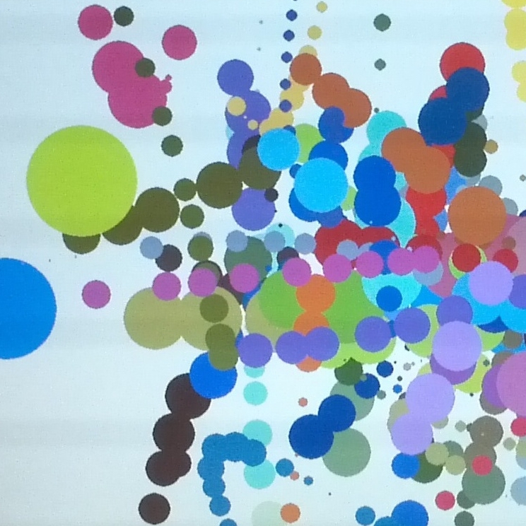
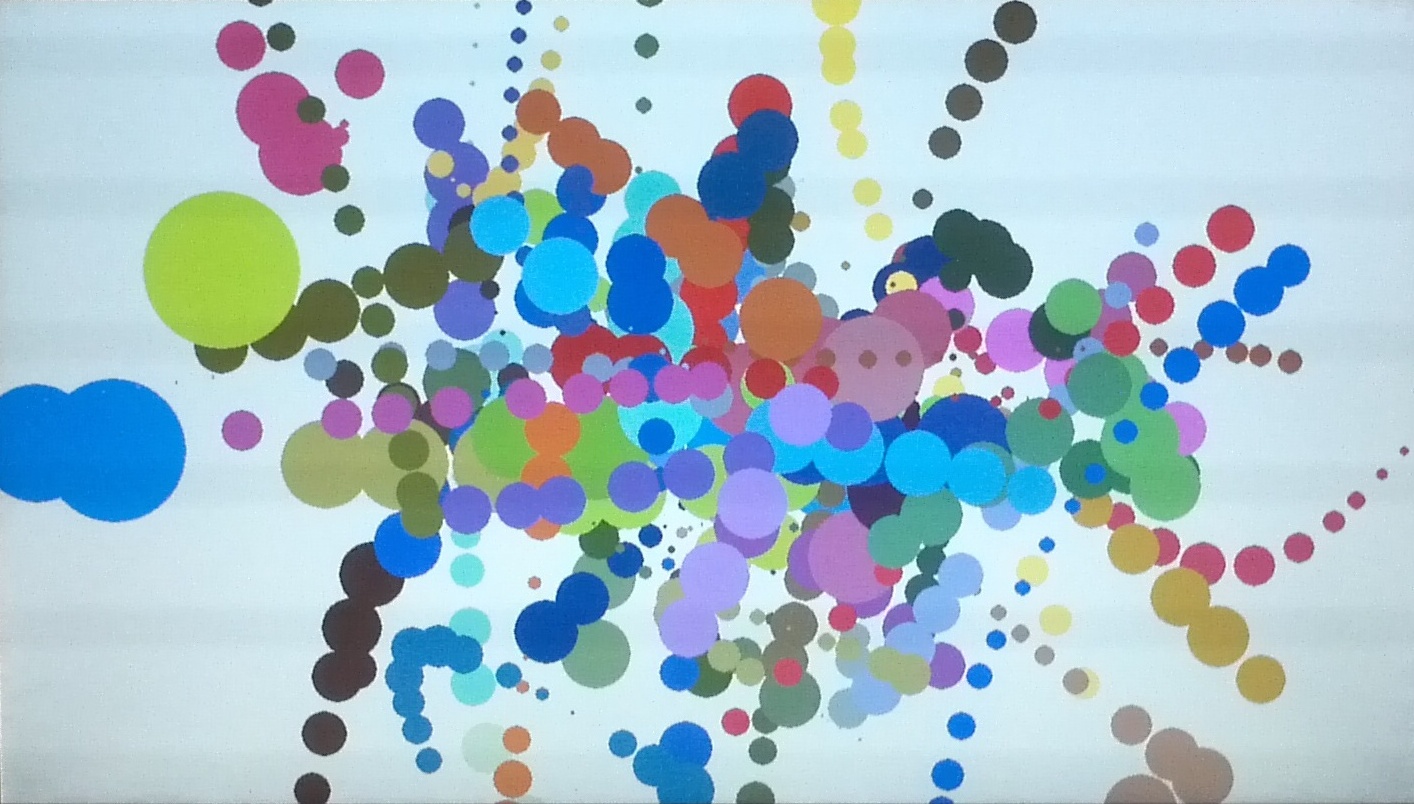
4. Art
Here's what we made together at the Ideas Bazaar...